USDM FSA LFP County Aggregations

Last
Update Repo
Size

This repository provides weekly US Drought Monitor (USDM) data aggregated to USDA Farm Service Agency Livestock Forage Program county boundaries. This dataset facilitates county-level analysis of drought conditions, supporting research, policy-making, and climate resilience planning.

📂 View the US Drought Monitor FSA LFP county archive listing here.

Federal law and FSA guidance describes a process by which county-level eligibility is determined by the intersection of county boundaries, the United States Drought Monitor weekly drought assessment, and the normal grazing period for each type of grazing land in each county.

The county data used in this repository were acquired via FOIA request 2025-FSA-08431-F by R. Kyle Bocinsky (Montana Climate Office) and fulfilled on September 8, 2025. The FOIA response, including the original Esri file geodatabase, is archived at https://sustainable-fsa.com/fsa-lfp-counties.

📈 About the US Drought Monitor (USDM)

The US Drought Monitor is a weekly map-based product that synthesizes multiple drought indicators into a single national assessment. It is produced by:

National Drought Mitigation Center (NDMC)
US Department of Agriculture (USDA)
National Oceanic and Atmospheric Administration (NOAA)

Each weekly map represents a combination of data analysis and expert interpretation.

The USDM weekly maps depicting drought conditions are categorized into six levels:

None: Normal or wet conditions
D0: Abnormally Dry
D1: Moderate Drought
D2: Severe Drought
D3: Extreme Drought
D4: Exceptional Drought

While USDM drought class boundaries are developed without regard to political boundaries, it is often aggregated by political boundaries to assist in decision-making and for regulatory purposes. This repository focuses on aggregating these data to the county level, enabling more localized analysis and decision-making.

Note: This archive is maintained by the Montana Climate Office, but all analytical authorship of the USDM drought maps belongs to the named USDM authors.

🗂 Directory Structure

usdm-counties-fsa-lfp.R: R script that processes and aggregates weekly USDM shapefiles to county boundaries.
usdm-counties-fsa-lfp.parquet: Processed county-level USDM data in a single parquet file.
usdm-counties-fsa-lfp.json: The worst drought class in each county each week, restructured for browsers (see Output Data below).
data/: Directory containing processed county-level USDM data.
README.Rmd: This README file, providing an overview and usage instructions.

The data/ directory and the consolidated Parquet are mirrored to S3 and served via CloudFront at https://data.sustainable-fsa.com/usdm-counties-fsa-lfp/ — that mirror is the archive of record, and the data are not kept in git. usdm-counties-fsa-lfp.json is a deliberate exception to that policy: it is mirrored to S3 and committed to git, so the web maps that read it have a small, versioned copy that moves with the repository.

Data Sources

USDM Polygons: Weekly .parquet files from sustainable-fsa/usdm
FSA LFP County Boundaries: Acquired via FOIA request 2025-FSA-08431-F.

USDM Polygons are reprojected to the same coordinate reference system as the FSA LFP County Boundaries, geometrically validated, and saved in .parquet format.

Processing Pipeline

The analysis pipeline is fully contained in usdm-counties-fsa-lfp.R and proceeds as follows:

Install and load dependencies:

Uses pak::pak() to ensure fresh, source-built installs of critical geospatial packages.

Download FSA LFP county boundary data. -Re-calculate county areas and save as data/fsa-lfp-counties.parquet
Download and intersect:

For each weekly USDM .parquet file:
Read county and drought geometries
Perform spatial intersection
Calculate the percent of each county area affected by each drought class
Tabular output is saved to data/usdm/USDM_{YYYY-MM-DD}.parquet

Output Structure: Each output file is a non-spatial .parquet file with the following fields:

STATEFP, State, COUNTYFP, County, CountyLSAD
usdm_date: The date of the USDM map
usdm_class: One of None, D0, D1, D2, D3, D4
usdm_percent: Proportion of the county in this drought class (as a decimal between 0 and 1)

Consolidate and publish:

Every weekly table is concatenated into usdm-counties-fsa-lfp.parquet, the archive of record.
The same records, reduced to the worst drought class per county and week, are written to usdm-counties-fsa-lfp.json for web maps (see Output Data below).

📤 Output Data

`usdm-counties-fsa-lfp.json`

The same weekly records as the Parquet — reduced from the identical table in the same run — restructured for direct use in a browser. It carries the worst drought class in each county each week and nothing else; the per-class area percents stay in the Parquet. It is what the web maps load, not an archive-of-record format: for analysis, use the Parquet.

One string per county: a county’s entire history is a single fixed-width string of class codes (0 = None through 5 = D4), one character per weekly USDM Tuesday on an implicit axis beginning 2000-01-04. No dates are stored, and a . marks a week in which the county is absent from the archive. The file is roughly 4.6 MB raw and about 400 KB gzipped over the wire.
Worst class, no threshold: the class for a county-week is the maximum over every record present, with no area-percent cutoff — any nonzero-area sliver of a class counts. This matches how fsa-lfp-eligibility-derived reads the archive.
Dictionary-coded names: county FIPS codes and county and state names each appear once, in arrays running parallel to the per-county strings.

The payload is self-describing via its schema field (usdm-max-class/1), a frozen contract with the web map: fields may be added, but existing ones are never renamed or reordered without bumping the schema. The same schema serves the usdm-counties and usdm-counties-reported archives; the dataset field says which of the three a given payload is.

🛠️ Dependencies

Key R packages used:

sf
terra
arrow
tidyverse
curl

The script installs all required packages using the pak package.

📍 Quick Start: Visualize a Weekly County USDM Map in R

This snippet shows how to load a weekly GeoParquet file from the archive and create a simple drought classification map using sf and ggplot2.

# Load required libraries
library(arrow)
library(sf)
library(ggplot2) # For plotting
library(tigris)  # For state boundaries
library(rmapshaper) # For innerlines function

## Get latest USDM data
latest <-
  jsonlite::fromJSON(
    "https://data.sustainable-fsa.com/usdm-counties-fsa-lfp/manifest.json"
  )$path |>
  stringr::str_subset("parquet") |>
  stringr::str_subset("data/usdm") |>
  max()
# e.g., [1] "data/usdm/USDM_2025-05-27.parquet"

date <-
  latest |>
  stringr::str_extract("\\d{4}-\\d{2}-\\d{2}") |>
  lubridate::as_date()

# Get the highest (worst) drought class in each county
usdm <-
  paste0("https://data.sustainable-fsa.com/usdm-counties-fsa-lfp/", latest) |>
  arrow::read_parquet() |>
  dplyr::group_by(STATEFP, COUNTYFP) |>
  dplyr::filter(usdm_class == max(usdm_class))

## Load the fsa-lfp-counties parquet file
counties <- 
  sf::read_sf("https://data.sustainable-fsa.com/usdm-counties-fsa-lfp/data/fsa-lfp-counties.parquet") |>
  # transform to WGS 84
  sf::st_transform("EPSG:4326") |>
  sf::st_cast("POLYGON", warn = FALSE, do_split = TRUE) |>
  tigris::shift_geometry() |>
  dplyr::group_by(STATEFP, COUNTYFP) |>
  dplyr::summarise(.groups = "drop") |>
  sf::st_cast("MULTIPOLYGON")

usdm_counties <-
  usdm |>
  dplyr::left_join(counties) |>
  sf::st_as_sf()

# Census counties for bounding box
census_counties <-
  tigris::counties(cb = TRUE,
                   resolution = "5m",
                   year = 2020,
                   progress_bar = FALSE) |>
  dplyr::filter(!(STATEFP %in% c("60", "66", "69", "78"))) %>%
  # transform to WGS 84
  sf::st_transform("EPSG:4326") |>
  sf::st_cast("POLYGON", warn = FALSE, do_split = TRUE) |>
  tigris::shift_geometry() |>
  dplyr::group_by(STATEFP, COUNTYFP) |>
  dplyr::summarise(.groups = "drop") |>
  sf::st_cast("MULTIPOLYGON")

# Plot the map
ggplot(counties) +
  geom_sf(data = sf::st_union(counties),
          fill = "grey80",
          color = NA) +
  geom_sf(data = usdm_counties,
          aes(fill = usdm_class), 
          color = NA) +
  geom_sf(data = rmapshaper::ms_innerlines(counties),
          fill = NA,
          color = "white",
          linewidth = 0.1) +
  geom_sf(data = counties |>
            dplyr::group_by(STATEFP) |>
            dplyr::summarise() |>
            rmapshaper::ms_innerlines(),
          fill = NA,
          color = "white",
          linewidth = 0.2) +
  scale_fill_manual(
    values = c("grey80",
               "#ffff00",
               "#fcd37f",
               "#ffaa00",
               "#e60000",
               "#730000"),
    drop = FALSE,
    name = "Drought\nClass") +
  labs(title = "US Drought Monitor",
       subtitle = format(date, " %B %d, %Y")) +
  coord_sf(
    xlim = sf::st_bbox(census_counties)[c("xmin", "xmax")],
    ylim = sf::st_bbox(census_counties)[c("ymin", "ymax")],
    clip = "off"
  ) +
  theme_void()

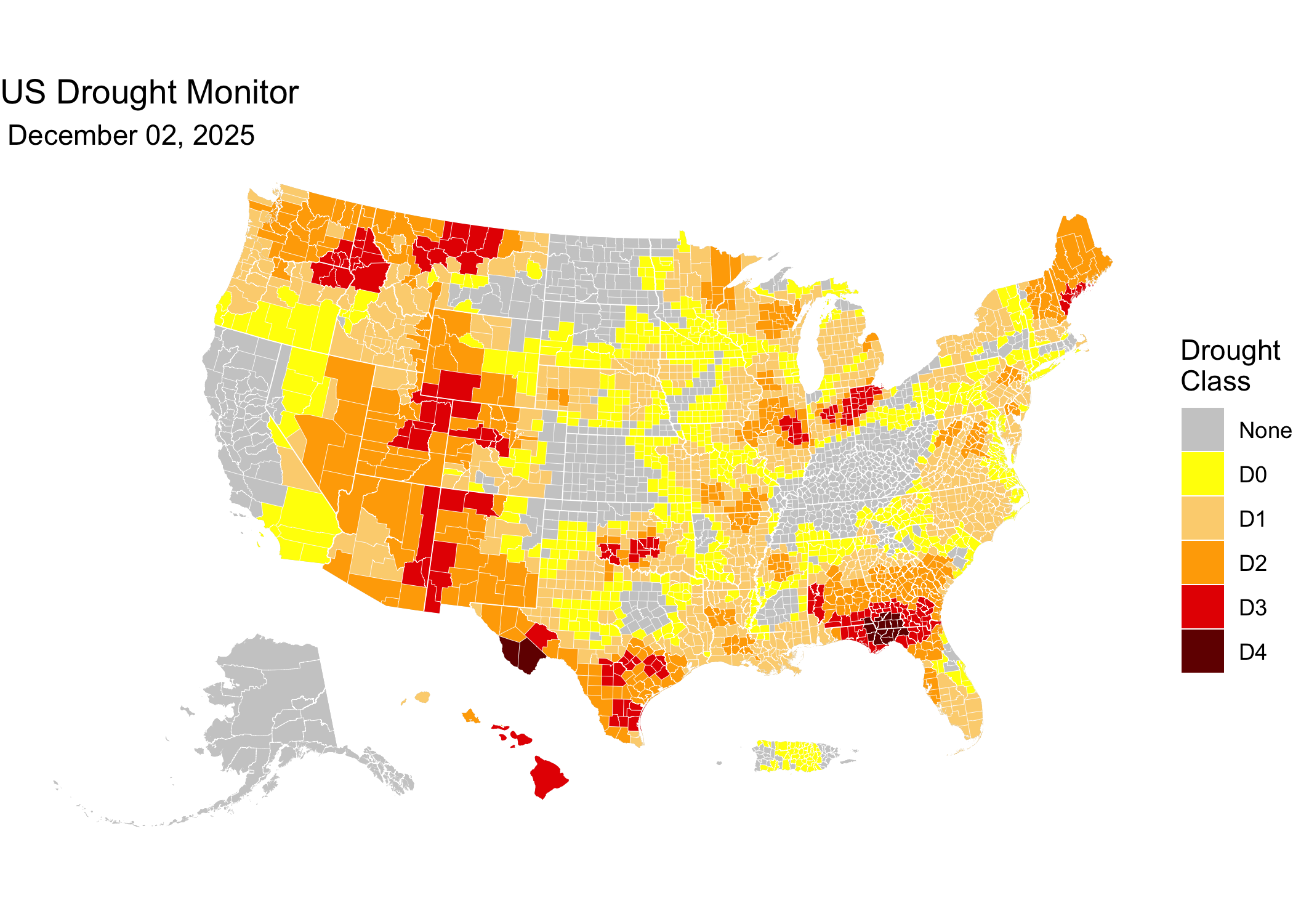
Latest USDM map date: September 01, 2026

📝 Citation

If you use this data in published work, please cite:

National Drought Mitigation Center, USDA, and NOAA. US Drought Monitor Weekly Maps Aggregated to FSA Livestock Forage Program County Boundaries. Aggregated, curated, and archived by R. Kyle Bocinsky, Montana Climate Office, University of Montana. Sustainable FSA project. Accessed YYYY-MM-DD. https://sustainable-fsa.com/usdm-counties-fsa-lfp/

Machine-readable metadata are in CITATION.cff; GitHub’s Cite this repository button (top right of the repo page) renders it as APA or BibTeX.

Acknowledgment: This work is part of the Enhancing Sustainable Disaster Relief in FSA Programs project, supported by the USDA Office of the Chief Economist, Office of Energy and Environmental Policy, and the USDA Climate Hubs.

📄 License

Raw USDM data (NDMC): Public Domain (17 USC § 105)

⚠️ Disclaimer

This dataset is archived for research and educational use only. The National Drought Mitigation Center hosts the US Drought Monitor. Please visit https://droughtmonitor.unl.edu.

👏 Acknowledgment

This project is part of:

Enhancing Sustainable Disaster Relief in FSA Programs
Supported by USDA OCE/OEEP and USDA Climate Hubs
Prepared by the Montana Climate Office

📬 Contact

R. Kyle Bocinsky
Director of Climate Extension
Montana Climate Office
📧 kyle.bocinsky@umontana.edu
🌐 https://climate.umt.edu