This repository provides a standardized archive of the US Department of Agriculture Farm Service Agency (FSA) Farm Payment Files. These files contain detailed records of payments made to agricultural program participants, originally released as Microsoft Excel files.

The included R script automates the discovery, download, and conversion of these files into a partitioned, analysis-ready format.

📁 Repository Contents

• fsa-payment-files.R: Main R script to download, extract, clean, and write the payment files to a partitioned Parquet format.
• README.Rmd: This file. Contains background information, usage instructions, and archive structure.
• data-raw/: Folder used for downloading and unpacking Excel and CSV files.
• fsa-payment-files/: Final output directory containing the processed data as a Parquet dataset, partitioned by state and year. When published to S3, this prefix also carries a _manifest.txt listing the HTTPS URL of every Parquet file (the leading underscore keeps Arrow’s dataset discovery from reading it as data).

🔁 Processing Workflow

The fsa-payment-files.R script performs the following steps:

1. Discovery: Scrapes the FSA payment files website to find downloadable Excel files (2004–2025).
2. Download: Saves original files to data-raw/.
3. Extraction: Parses each Excel file, handling annual variation in schema and formatting.
4. Standardization: Renames fields, standardizes formats (e.g., FIPS codes, program names), and removes duplicates.
5. Archiving: Writes the full dataset to the fsa-payment-files/ directory as partitioned Parquet files (State FSA Name= and Accounting Program Year= directories).
6. Upload (optional): Syncs the Parquet archive to a public S3 bucket with the AWS CLI (aws s3 sync), verifies the remote listing matches the local build, and publishes a _manifest.txt of HTTPS URLs for access via the CloudFront portal.

☁️ Public Access via S3

The full archive is hosted in a public Amazon S3 bucket:

s3://sustainable-fsa/fsa-payment-files/

You can access the data directly using:

AWS CLI

aws s3 ls s3://sustainable-fsa/fsa-payment-files/ --no-sign-request

In R with arrow (recommended)

library(arrow)

## 
## Attaching package: 'arrow'

## The following object is masked from 'package:utils':
## 
##     timestamp

bucket <- s3_bucket("sustainable-fsa", anonymous = TRUE, region = "us-west-2")

dataset <- open_dataset(bucket$path("fsa-payment-files"))

dataset

## FileSystemDataset with 1642 Parquet files
## 16 columns
## County FSA Name: dictionary<values=string, indices=int16>
## FSA Code: dictionary<values=string, indices=int16>
## Accounting Program Code: string
## Accounting Program Description: string
## Payment Date: date32[day]
## Disbursement Amount: double
## Formatted Payee Name: string
## Address Information Line: string
## Delivery Address Line: string
## City Name: string
## State Abbreviation: string
## Zip Code: string
## Delivery Point Bar Code: string
## Source File: dictionary<values=string, indices=int16>
## State FSA Name: string
## Accounting Program Year: int32

Queries that filter on the partition columns (State FSA Name, Accounting Program Year) only download the matching Parquet files. Arrow decodes the partition values for you, so filters use plain names — e.g., dplyr::filter(\State FSA Name` == “New Mexico”)`.

🌐 Public Access via HTTPS (CloudFront)

The same archive is served over plain HTTPS at:

https://data.sustainable-fsa.com/fsa-payment-files/

HTTPS has no directory listing, so a manifest of every file URL is published at _manifest.txt (regenerated on every data update). DuckDB’s httpfs extension can query these URLs directly — and filters on the hive partition columns are applied to the URL paths before any file is fetched, so you keep the benefits of the partitioning without S3 access:

library(DBI)

manifest <- readLines("https://data.sustainable-fsa.com/fsa-payment-files/_manifest.txt")

con <- dbConnect(duckdb::duckdb())
invisible(dbExecute(con, "INSTALL httpfs; LOAD httpfs;"))

files_sql <- paste0("[", paste0("'", manifest, "'", collapse = ",\n"), "]")

lfp_mt <- dbGetQuery(con, glue::glue('
  SELECT "Accounting%20Program%20Year" AS "Accounting Program Year",
         SUM("Disbursement Amount") AS "Disbursement Amount"
  FROM read_parquet({files_sql}, hive_partitioning = true)
  WHERE "State%20FSA%20Name" = \'Montana\'
  GROUP BY 1
  ORDER BY 1
'))

dbDisconnect(con, shutdown = TRUE)

tail(lfp_mt)

##    Accounting Program Year Disbursement Amount
## 26                    2021           564897706
## 27                    2022           251931734
## 28                    2023           130575231
## 29                    2024           435473337
## 30                    2025            57473319
## 31                      NA            45995811

Notes for DuckDB users:

• Because these URLs are percent-encoded, the hive column names surface encoded — "State%20FSA%20Name" and "Accounting%20Program%20Year" (quote them with double quotes in SQL) — and multi-word partition values keep one layer of encoding, so filters need encoded literals (e.g., WHERE "State%20FSA%20Name" = 'New%20Mexico'). Use DuckDB’s url_decode() to clean values for display.
• "Accounting%20Program%20Year" autocasts to an integer. A few partitions hold rows with malformed years in the source files: __HIVE_DEFAULT_PARTITION__ (surfaces as NULL) and 0 — filter them out if they matter for your analysis.
• For simple cases you can skip the SQL-side filter entirely and subset the manifest in R first, e.g. manifest[grepl("Name=Montana/", manifest, fixed = TRUE)].
• DuckDB can also query the S3 bucket directly — no manifest needed, and here the column names and values come through clean ("State FSA Name", 'New Mexico'):

con <- dbConnect(duckdb::duckdb())
dbExecute(con, "INSTALL httpfs; LOAD httpfs;")
dbExecute(con, "CREATE SECRET (TYPE s3, PROVIDER config, REGION 'us-west-2');")
dbGetQuery(con, '
  SELECT "County FSA Name", SUM("Disbursement Amount") AS total
  FROM read_parquet(\'s3://sustainable-fsa/fsa-payment-files/*/*/*.parquet\',
                    hive_partitioning = true)
  WHERE "State FSA Name" = \'Montana\'
  GROUP BY 1 ORDER BY total DESC LIMIT 10')

🧭 Notes

• File structure varies by year, and the script includes heuristics to detect column shifts and missing headers.
• Partitioning by state and year facilitates fast querying and cloud-native workflows.
• The processing script can be rerun to include new years as they are released.

📅 Update Schedule

This dataset is refreshed annually after the USDA FSA releases new payment files, typically in the spring. Additional years or corrections may be processed as available.

🔗 Related Resources

• USDA FSA FOIA Payment Page
• Arrow and Parquet in R

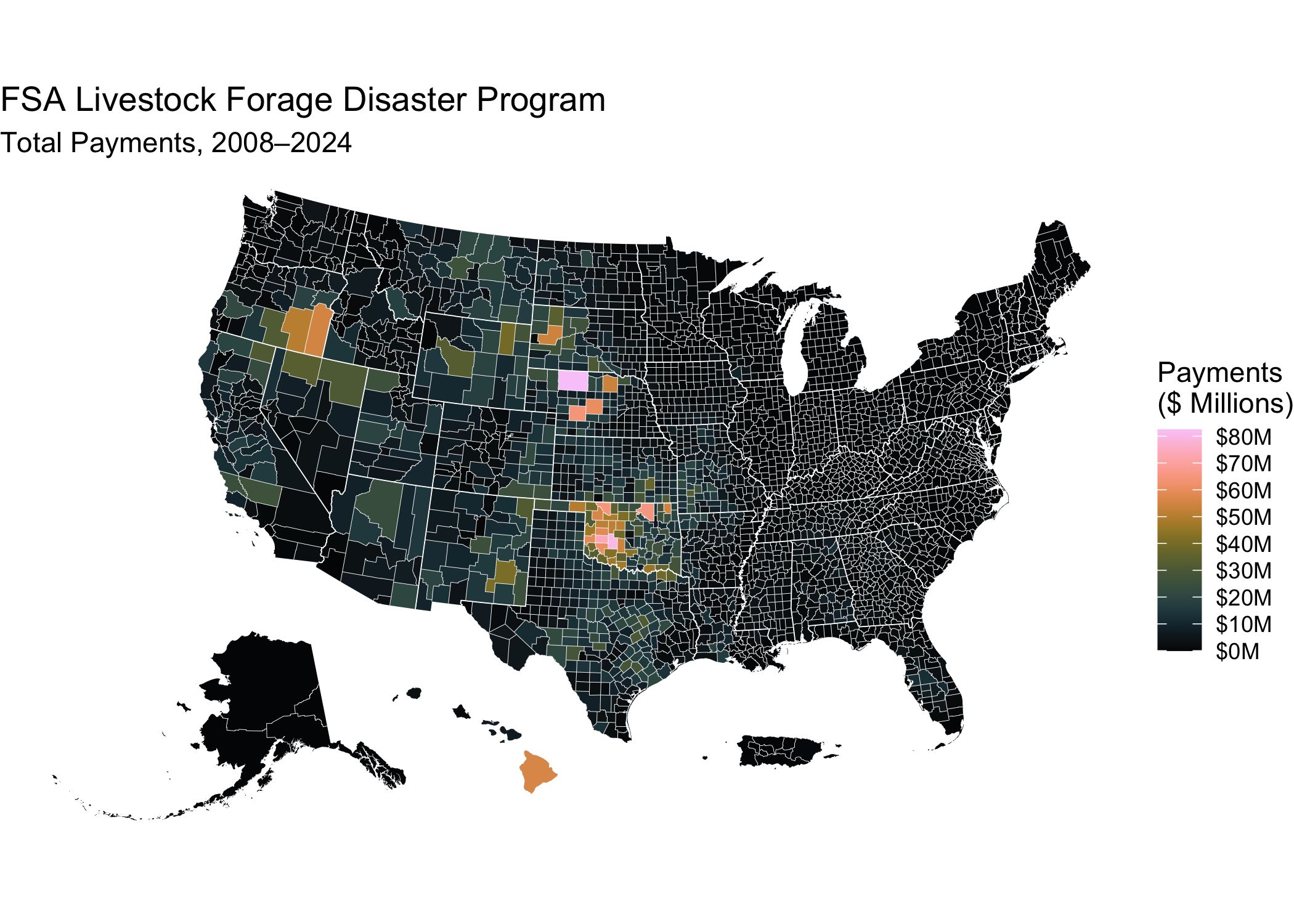
📍 Quick Start: Visualize data in the FSA Farm Payment Files in R

This snippet shows how to load data from the Farm Payment Files archive and create a simple map using sf and ggplot2.

# Load required libraries
library(arrow)
library(sf)
library(ggplot2) # For plotting
library(tigris)  # For state boundaries
library(rmapshaper) # For innerlines function

# Example accessing payment files on S3
# A map of 2025 LFP Payments by county

lfp_payments <-
  # To run this from anywhere, open the dataset from S3 instead:
  # arrow::s3_bucket("sustainable-fsa", anonymous = TRUE,
  #                  region = "us-west-2")$path("fsa-payment-files") |>
  "fsa-payment-files" |>
  arrow::open_dataset() |>
  dplyr::filter(`Accounting Program Description` %in% 
                  c(
                    "LIVESTOCK FORAGE PROGRAM",
                    "LIVESTOCK FORAGE DISASTER PROGRAM",
                    "LIVESTOCK FORAGE DISASTER PROGRAM (COF)"
                  )) |>
  dplyr::group_by(`FSA Code`) |>
  dplyr::summarise(
    `Disbursement Amount` = sum(`Disbursement Amount`, na.rm = TRUE)
  ) |>
  dplyr::collect()

## Download from the FSA_Counties_dd17 archive
counties <- 
  sf::read_sf("https://data.sustainable-fsa.com/fsa-counties-dd17/fsa-counties-dd17.topojson",
              layer = "counties") |>
  sf::st_set_crs("EPSG:4326") |>
  sf::st_transform("EPSG:5070")

lfp_payments_counties <-
  lfp_payments |>
  dplyr::select(id = `FSA Code`,
                `Disbursement Amount`) |>
  dplyr::right_join(counties) |>
  sf::st_as_sf() |>
  dplyr::mutate(
    `Disbursement Amount` = 
      tidyr::replace_na(`Disbursement Amount`, 0)
  )


# Plot the map
ggplot(counties) +
  geom_sf(data = sf::st_union(counties),
          fill = "grey80",
          color = NA) +
  geom_sf(data = lfp_payments_counties,
          aes(fill = `Disbursement Amount`), 
          color = NA) +
  geom_sf(data = rmapshaper::ms_innerlines(counties),
          fill = NA,
          color = "white",
          linewidth = 0.1) +
  geom_sf(data = counties |>
            dplyr::group_by(state) |>
            dplyr::summarise() |>
            rmapshaper::ms_innerlines(),
          fill = NA,
          color = "white",
          linewidth = 0.2) +
  scale_fill_viridis_c(#palette = "OrRd",
    option = "turbo",
    direction = 1,
    na.value = "grey80",
    limits = c(0,100000000),
    breaks = c(0,10000,100000,1000000,10000000, 100000000),
    trans = scales::pseudo_log_trans(sigma = 1000),
    labels=scales::label_currency(scale_cut = scales::cut_short_scale()),
    name = 
      paste0(
        "Livestock Forage Program Payments, 2008–2025\nTotal: ",  
        scales:::dollar(sum(lfp_payments_counties$`Disbursement Amount`, na.rm = TRUE)),
        " as of ", format(lubridate::today(), "%B %d, %Y")
      ),
    guide = guide_colorbar(title.position = "top") ) +
  theme_void(base_size = 24) +
  theme(legend.position = "bottom",
        legend.justification = "center",
        legend.key.width = unit(0.15, "npc"),
        legend.title = element_text(size = 16, hjust = 0.5),
        legend.text = element_text(size = 14, hjust = 0.5),
        strip.text.x = element_text(margin = margin(b = 5)),
        strip.text.y = element_text(margin = margin(r = 5)))

🧭 About FSA County Codes

The USDA FSA uses custom county definitions that differ from standard ANSI/FIPS codes used by the U.S. Census. To align the Farm Payment Files with geographic boundaries, use the FSA-specific geospatial dataset archived in the companion repository:

🔗 sustainable-fsa/fsa-counties-dd17

FSA county codes are documented in FSA Handbook 1-CM, Exhibit 101.

📝 Citation

If you use this data in published work, please cite:

USDA Farm Service Agency. Farm Payment Files, 2004–2025. Curated and archived by R. Kyle Bocinsky, Montana Climate Office, University of Montana. Sustainable FSA project. Accessed YYYY-MM-DD. https://sustainable-fsa.com/fsa-payment-files/

Machine-readable metadata are in CITATION.cff; GitHub’s Cite this repository button (top right of the repo page) renders it as APA or BibTeX.

Acknowledgment: This work is part of the Enhancing Sustainable Disaster Relief in FSA Programs project, supported by the USDA Office of the Chief Economist, Office of Energy and Environmental Policy, and the USDA Climate Hubs.

📄 License

• Raw FSA Farm Payment Files data (USDA): Public Domain (17 USC § 105)
• Processed data & scripts: © R. Kyle Bocinsky, released under CC0 and MIT License as applicable

⚠️ Disclaimer

This dataset is archived for research and educational use only. It may not reflect current FSA payments and policy. Always consult your local FSA office for the latest program guidance.

To locate your nearest USDA Farm Service Agency office, use the USDA Service Center Locator:

🔗 USDA Service Center Locator

👏 Acknowledgment

This project is part of:

Enhancing Sustainable Disaster Relief in FSA Programs
Supported by USDA OCE/OEEP and USDA Climate Hubs
Prepared by the Montana Climate Office

📬 Contact

R. Kyle Bocinsky
Director of Climate Extension
Montana Climate Office
📧 kyle.bocinsky@umontana.edu
🌐 https://climate.umt.edu